What follows are my attempts at solving exercises at the end of chapter 2 from Reinforcement Learning: An Introduction. Exercise 2.1 asks us, which would work the best when using -greedy action selection, one of action-value methods described in the book. We can reconstruct the original setup with the following code.
import numpy as np
import matplotlib.pyplot as plt
rng = np.random.default_rng()
num_bandits = 2000
num_arms = 10
rewards = []
for bandit in range(num_bandits):
rewards.append(rng.normal(0, 1, num_arms))
testbed = np.array(rewards)
# -----------------------------------------------------------------
num_steps = 1000
epsilons = [0, 0.01, 0.1]
results = {}
for epsilon in epsilons:
avg_rewards = np.zeros(num_steps)
optimal_actions = np.zeros(num_steps)
for bandit in range(num_bandits):
Q = np.zeros(num_arms)
N = np.zeros(num_arms)
optimal = np.argmax(testbed[bandit]) # true best arm
for t in range(num_steps):
if rng.random() < epsilon:
a = rng.integers(num_arms)
else:
a = np.argmax(Q)
r = testbed[bandit, a] + rng.normal(0, 1)
N[a] += 1
Q[a] += (r - Q[a]) / N[a]
avg_rewards[t] += r
optimal_actions[t] += (a == optimal)
results[epsilon] = {
'rewards': avg_rewards / num_bandits,
'optimal': optimal_actions / num_bandits * 100
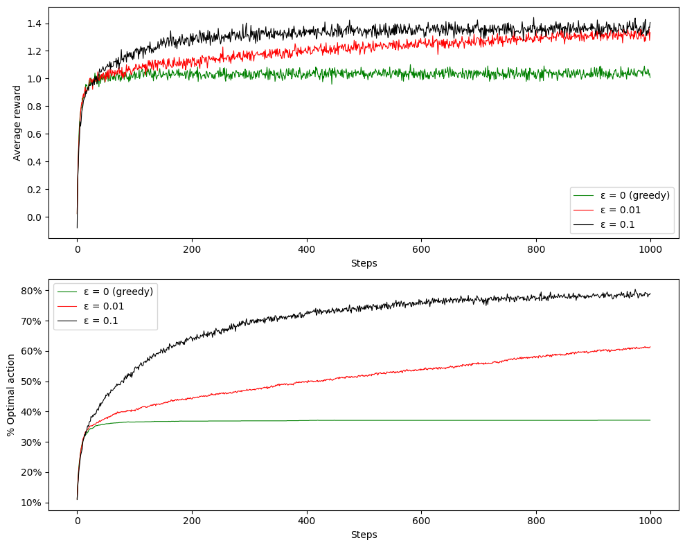
}Plotting the results gives plots similar to Figure 2.1 of the book. Here we can see, that =0.1 performs best for the 1000 steps, since it has the highest average reward. However, from a long-term point of view, =0.01 will by the book work better. Selecting the optimal action has probability at least , which is 99%.
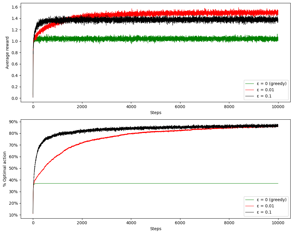
 Running the algorithm again for 10000 steps manifest how the average reward becomes higher after around 2000 steps, although it run for significantly larger amount of time. This is also good example of the exploration-exploitation tradeoff.
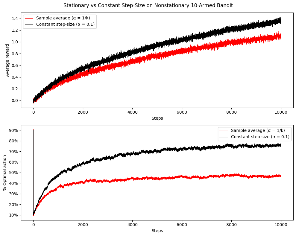
Following with the programming exercise, we are asked to change the previous setup to a nonstationary problem. The book introduced another variant next to average sampling with a constant step-size . We should compare these two value estimate methods, while still selecting action with -greedy algorithm. The books asks us to initiate all bandits and their bandit rewards to the same value. I choose 0, even though other values are possible (like some positive constant, which is addressed as optimistic initial setup). After each step, we should perform a random walk - adding a random number from a neighborhood. In order to not perform large drifts from previous action values, I’m adding samples from . The code is almost the same, but the optimal action is rediscovered after each step and the way of computing immediate reward is a bit different for constant .
rng = np.random.default_rng()
num_bandits = 2000
num_arms = 10
num_steps = 10000
epsilon = 0.1
alpha = 0.1

testbed = np.zeros((num_bandits, num_arms))

avg_rewards = {
	'sample_average': np.zeros(num_steps),
	'constant': np.zeros(num_steps)
}

optimal_actions = {
	'sample_average': np.zeros(num_steps),
	'constant': np.zeros(num_steps)
}

for bandit in range(num_bandits):
	Q_avg = np.zeros(num_arms)
	Q_const = np.zeros(num_arms)
	N_avg = np.zeros(num_arms)
	N_const = np.zeros(num_arms)

	for t in range(num_steps):
		# action selection
		if rng.random() < epsilon:
			a_avg = rng.integers(num_arms)
		else:
			a_avg = np.argmax(Q_avg)

		if rng.random() < epsilon:
			a_const = rng.integers(num_arms)
		else:
			a_const = np.argmax(Q_const)

		optimal = np.argmax(testbed[bandit])

		r_avg = testbed[bandit, a_avg] + rng.normal(0, 1)
		r_const = testbed[bandit, a_const] + rng.normal(0, 1)

		N_avg[a_avg] += 1
		Q_avg[a_avg] += (r_avg - Q_avg[a_avg]) / N_avg[a_avg]
		Q_const[a_const] += alpha * (r_const - Q_const[a_const])

		# random walk
		testbed[bandit] += rng.normal(0, 0.01, num_arms)

		avg_rewards['sample_average'][t] += r_avg
		avg_rewards['constant'][t] += r_const
		optimal_actions['sample_average'][t] += (a_avg == optimal)
		optimal_actions['constant'][t] += (a_const == optimal)

results = {
	'sample_average': {
		'rewards': avg_rewards['sample_average'] / num_bandits,
		'optimal': optimal_actions['sample_average'] / num_bandits * 100
	},
	'constant': {
		'rewards': avg_rewards['constant'] / num_bandits,
		'optimal': optimal_actions['constant'] / num_bandits * 100
	}
}
After plotting the results, we can see how the average reward keeps growing, but optimal action being stagnant. The sample average weights all the rewards equally and doesn’t adapt to recent changes. The constant step-size gives more weight to the last actions rewards and it tends to explore even after sample average starts to only exploit.